Quick start guide to model building and running with SPyice

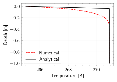
Demonstrates a simple example for a freezing sea ice model for a simple heat diffusion setup with default settings of initial conditions of 265K at the top boundary and Salinity of 34ppt choosing constant fixed Dirichlet boundary conditions. For the one phase distinct interface system where sea water is at melt temperature of 271.25K.

Import Packages

import os
from pathlib import Path
import matplotlib.pyplot as plt

%matplotlib inline
from omegaconf import OmegaConf

from spyice.utils import create_output_directory
from spyice.postprocess import Analysis, VisualiseModel
from spyice.utils import ConfigSort
from spyice.models import SeaIceModel
from spyice.preprocess import PreProcess

Define Inputs and Project Output paths

# creates a OmegaConf object from a dictionary for fast testing only for parameters: constants, dt, S_IC, iter_max, dz
constants_dict = {
    "constants": {"constants": "real"},
    "dt": {"dt": 47},
    "S_IC": {"S_IC": "S34"},
    "iter_max": {"iter_max": 1500},
    "dz": {"dz": 0.01},
}
config_raw = OmegaConf.create(constants_dict)
config = ConfigSort.getconfig_dataclass(config_raw, config_type="jupyter")

# choose your output directory
base_dir = Path.cwd()
output_base_dir = Path(base_dir, "output")
wo_hydra_dir = Path(output_base_dir, "without_hydra")
out_dir_final = create_output_directory(wo_hydra_dir, config.initial_salinity.S_IC, "2", "0.01", "47", "1500", "example")

Preprocessing

# preprocess the data
preprocess_data, userinput_data = PreProcess.get_variables(config_raw, out_dir_final)

Preprocessing...
User Configuration Data Setup Complete...
Geometry Data Setup Complete...
Results Data Setup Complete...
Time step set to: 47s
Applied Initial & Boundary Conditions...
Preprocessing done.

Run model

# run the model
results_data = SeaIceModel.get_results(preprocess_data, userinput_data)
analysis_data = Analysis.get_error_results(
            t_k_diff=results_data.t_k_diff,
            t_stefan_diff=results_data.t_stefan_diff,
            residual=results_data.residual_voller_all,
            temperature_mushy=results_data.t_k_iter_all,
            phi_mushy=results_data.all_phi_iter_all,
            salinity_mushy=results_data.s_k_iter_all,
            output_dir=out_dir_final,
        )

Running model...
Model run complete and Ready for Analysis.
Running error analysis...
Calculating errors...
Residuals exported successfully.

Visualization of Model:

for more info on other visualization options look at: visualize model

model_visualization_object = VisualiseModel(
    user_input_dataclass=userinput_data,
    results_dataclass=results_data,
    error_analysis_dataclass=analysis_data,
)

Visualisation object created...

%matplotlib inline
model_visualization_object.plot_temperature_heatmap(savefig=True, export_csv=False)

Plotting Temperature heatmap...