Implementation basics

caption

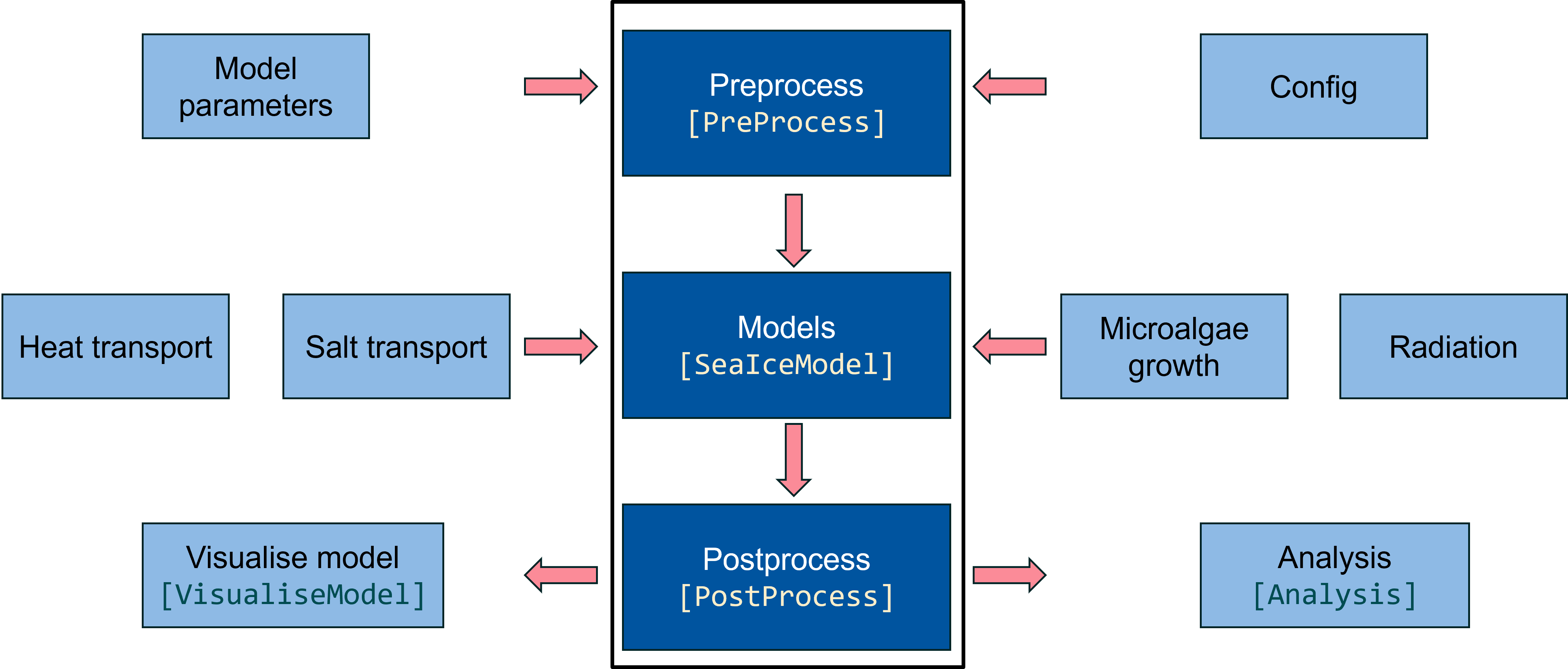
The inputs are initialised and processed by the Prepossessing class. Here the respective initial and boundary conditions are applied to the user-defined discrete finite difference mesh. The simulation model is executed for the given number of maximum iterations which allows to model for a time period of (time step size) * (max iterations). At a given time \($t$\), the numerical model is solved until it attains a convergence for field parameters temperature, salinity and volumetric liquid fraction whose pseudo code is given below in code_pseudo:

Python example

def run_model(self) -> None:
    """Runs the model using the provided configuration and output directory."""
    # apply boundary and initial conditions during the pre-processing stage and get the pre-processed dataclass
    preprocess_data, userinput_data = PreProcess.get_variables(
        self.config, self.out_dir_final
    )
    # run the sea ice model and get the results dataclass
    results_data = SeaIceModel.get_results(preprocess_data, userinput_data)
    # error analysis of results and get the analysis dataclass
    analysis_data = Analysis.get_error_results(
        t_k_diff=results_data.t_k_diff, t_stefan_diff=results_data.t_stefan_diff
    )
    # plot the sea ice model using the user input, results, and analysis dataclasses
    self.plot_model(userinput_data, results_data, analysis_data)

Once the field values are obtained, an error analysis is performed using Analytical class to verify discrepancies between numerical and analytical results. The analytical results are verified with the one-phase Stefan problem which keeps one of the two phases constant (liquid phase in this project) while modelling. The temperature field can be visualised using the Visualisemodel class where the temperature fields can be compared at different spatial nodes points and their nodal time evolution in comparison to the analytical results.